6. [Python] Image Compression
PCA, SVD, DCT 등으로 이미지의 주요 정보만 사용해서 나타내는 방법을 알아보기.
DCT는 JPEG, H.264 등 주요 영상 압축 알고리즘에 사용된다.
1. PCA
- 영상 신호에서 주성분을 뽑아낸다.
- h,w의 영상신호이면 주성분은 최대 min(h,w)개를 가질 수 있다.
- 이 주성분들 중 major한 feature만 사용하고, 나머지 주성분은 사용하지 않고 이미지를 복원한다.
y,cr,cb = cv2.split(img_ycrcb)

h,w= y.shape

k = 30
pca = PCA(n_components=k)
y_pca = pca.fit_transform(y)
y_ipca = pca.inverse_transform(y_pca)
y_ipca = np.clip(y_ipca, 0, 255).astype(np.uint8)

img_pca_comp = cv2.merge([y_ipca, cr, cb])
img_pca_comp = cv2.cvtColor(img_pca_comp, cv2.COLOR_YCrCb2RGB)

fig,ax = plt.subplots(1,2,figsize=(8,8))
images = [img, img_pca_comp]
titles = ['Origin', f'PCA Image (Components : {k})']

for idx, (image,title) in enumerate(zip(images, titles)):
    ax[idx].imshow(image)
    ax[idx].set_title(title)
    ax[idx].axis('off')

plt.tight_layout()
plt.show()
explained_variance = pca.explained_variance_ratio_
cumulative_explained_variance = np.cumsum(explained_variance)

fig,ax = plt.subplots(figsize=(6,4))
ax.plot(range(1,k+1), explained_variance, marker='o', linestyle='-', color='royalblue', label='Explained Variance')
ax.plot(range(1,k+1), cumulative_explained_variance, marker='o', linestyle='-', color='tomato', label='Cumulative Explained Variance')
ax.set_xlabel('Principal Components')
ax.set_ylabel('Explained Variance Ratio')
ax.set_title('Explained Variance Ratio')
ax.set_ylim([-0.05,1])
ax.legend(loc='right')
plt.tight_layout()
plt.show()
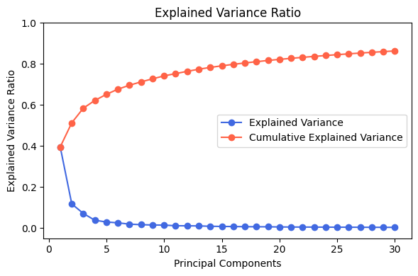
- threshold를 통해서 특정 퍼센티지가 넘어가는 변수까지만 선택하는 방법이 일반적이다.
- 보통 설명변수가 0.8정도가 되면 원본 이미지의 정보를 대부분 담고있다.
- 0.9정도가 되면 거의 차이가 없다.
2. SVD
- 행렬을 3개의 행렬로 분해한다.
- 대각행렬의 상위 x개의 feature를 사용해서 영상을 압축한다.
y,cr,cb = cv2.split(img_ycrcb)

k = 1
img_svd = np.linalg.svd(y, full_matrices=False)
U,S,VT = img_svd
S = np.diag(S)
U_k = U[:,:k]
S_k = S[:k,:k]
VT_k = VT[:k,:]

img_isvd = np.dot(U_k, np.dot(S_k, VT_k))
img_isvd = np.clip(img_isvd, 0, 255).astype(np.uint8)

img_svd_comp = cv2.merge([y_ipca, cr, cb])
img_svd_comp = cv2.cvtColor(img_svd_comp, cv2.COLOR_YCrCb2RGB)

images = [img, img_svd_comp]
titles = ['Origin', f'SVD Image (Components : {k})']

fig,ax = plt.subplots(1,2,figsize=(8,8))
for idx, (image,title) in enumerate(zip(images, titles)):
    ax[idx].imshow(image)
    ax[idx].set_title(title)
    ax[idx].axis('off')

plt.tight_layout()
plt.show()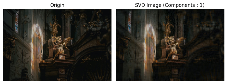
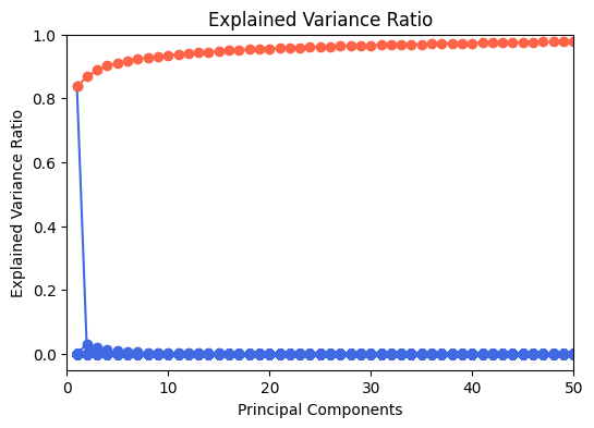
- PCA와 다르게 기본적으로 하나의 특이값만 사용해도 굉장히 많은 정보를 포함한다.
explained_variance = (S**2) / np.sum(S**2)
temp = np.array([sum(v) for v in explained_variance])
temp[k:] = 0
cumulative_explained_variance = np.cumsum(temp)

fig,ax = plt.subplots(figsize=(6,4))
ax.plot(range(1, min(h,w)+1), explained_variance, color='royalblue', marker='o', label='Explained Variance')
ax.plot(range(1, min(h,w)+1), cumulative_explained_variance, color='tomato', marker='o', label='Cumulative Explained Variance')
ax.set_xlabel('Principal Components')
ax.set_ylabel('Explained Variance Ratio')
ax.set_title('Explained Variance Ratio')
ax.set_xlim([0,k])
ax.set_ylim([-0.05,1])
plt.show()
3. DCT
- cosine transform을 이용한다.
- Frequency Domain으로의 번환이므로 고주파 대역의 정보를 날려서 데이터를 압축한다.\
- 고주파 대역이 차지하는 정보는 많지만, 이미지에서는 차이가 크게 나지 않는다.
def DCT(img):
    return cv2.dct(np.float32(img))

def IDCT(img_dct):
    return cv2.idct(img_dct).astype(np.uint8)

def magnitude(img_dct):
    magnitude = 20 * np.log(np.abs(img_dct) + 1)
    return magnitude

def get_mask(img_dct, cutoff: int):
    h, w = img_dct.shape
    ratio = np.sqrt(cutoff/100)
    mask = np.zeros((h,w), np.float32)
    mask[:int(h*ratio), :int(w*ratio)] = 1
    return mask

y,cr,cb = cv2.split(img_ycrcb)
img_dct = DCT(y)

img_dct_masked = img_dct * get_mask(img_dct,10)
img_reconstrunted = cv2.merge([IDCT(img_dct_masked),cr,cb])
img_reconstrunted = cv2.cvtColor(img_reconstrunted,cv2.COLOR_YCrCb2RGB)


fig, ax = plt.subplots(2,2, figsize=(8,8))
images = [img, magnitude(img_dct), img_reconstrunted, magnitude(img_dct_masked)]
titles = ['Original Image', 'DCT Image', 'Reconstructed Image', 'Masked DCT Image']

for idx, (image,title) in enumerate(zip(images, titles)):
    h,w = divmod(idx,2)
    ax[h,w].imshow(image, cmap='magma' if 'DCT' in title else None)
    ax[h,w].set_title(title)
    ax[h,w].axis('off')

plt.tight_layout()
plt.show()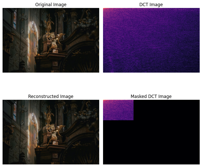
- DCT 영역에서 저주파 10%만 가져와도 영상의 대부분을 무리없이 확인할 수 있다.
- 디테일한 정보들이 없어지지만, 이미지의 형태는 5~10프로만 되도 확인가능하다.
'Machine Learning > Image Processing' 카테고리의 다른 글
| 9. [Python] Image Transform (0) | 2022.08.25 |
|---|---|
| 8. [Python] Morpological Transfomation (0) | 2022.08.15 |
| 7. [Python] Thresholding (0) | 2022.08.08 |
| 5. [Python] Histogram Modeling (0) | 2022.07.28 |
| 4. [Python] Frequency Domain (0) | 2022.07.22 |
| 3. [Python] Spatial Domain (0) | 2022.07.13 |
| 2. [Python] Color Channel (0) | 2022.07.13 |


댓글